Build a 2026 Residential Solar Simulator: Calculate Output Gains from Bifacial Panels and AI-Tracking vs Standard TOPCon Panels
A spreadsheet-grade, step-by-step simulation you can build in an afternoon — with the derate chain, albedo tables, and tracking-gain math we actually use to quote systems.
Every solar quote starts with the same lie: the nameplate. A "450W panel" produces 450 watts in a lab at 25°C cell temperature under a calibrated sun — conditions your roof will see maybe twice a year, in passing. What your system actually delivers depends on temperature, soiling, inverter losses, shading, orientation, and two technologies that are reshaping residential math in 2026: bifacial modules that harvest reflected light off the surface behind them, and AI-driven tracking that follows the sun instead of sitting fixed. This guide builds you a working output simulator — a structured calculation you can run in any spreadsheet — so you can quantify exactly what those upgrades are worth on your site before spending a dollar.
We run versions of this math every day when quoting systems at PES Supply. The model below is deliberately transparent: every factor is a number you can see, adjust, and defend. It's not a black-box app — it's the same derate chain the industry-standard tools use under the hood, simplified to residential scale. You'll need about an hour, your site's latitude and average weather, and the spec sheets of the panels you're comparing. Let's build it.
Start with the reference case: a fixed-tilt, south-facing residential array of modern n-type TOPCon modules — the current mainstream premium technology, well represented in our n-type panel collection by products like the Silfab Elite N-Type TOPCon and its all-black 370W sibling. The core simulation equation is simple:
Annual kWh = Array kW (DC) × Peak Sun Hours/day × 365 × Total Derate Factor
The art is in the derate chain. Each loss multiplies the next — they compound, they don't add. Here's the chain we use, with realistic 2026 values for a well-installed residential system:
| Derate Factor | Typical Value | What Drives It |
|---|---|---|
| Irradiance on tilted plane (POA transposition) | 1.00–1.08 (tilt ≈ latitude) | Optimized tilt gains a few % over horizontal |
| Azimuth loss (vs true south) | 0.95–1.00 | SE/SW costs 2–4%; E/W costs 10–15% |
| Soiling | 0.95–0.98 | Dust, pollen, bird traffic; rain-washed roofs run high |
| Shading | 0.90–1.00 | Site-specific; measure with a shade tool, don't guess |
| Temperature loss | 0.88–0.95 | Cell temp × coefficient — the big one, detailed below |
| Module mismatch + wiring (DC) | 0.97–0.98 | String variation, connector losses |
| Inverter efficiency | 0.96–0.98 | CEC weighted efficiency on the datasheet |
| AC wiring + availability | 0.98–0.99 | Homerun losses, downtime |
| Total derate (multiply all) | ≈ 0.74–0.86 typical; 0.80 is a defensible default | Honest systems land here |
Worked example — the baseline for everything below: 8 kW DC of TOPCon, a US-average 4.5 peak sun hours, 0.80 derate: 8 × 4.5 × 365 × 0.80 = 10,512 kWh/year. If your quote promises 12,000+ from that array on that site, someone's derate chain is fantasy. Build yours factor by factor and you have a quote-checking superpower. For nameplate-to-system sizing, our system size calculator and inverter sizing calculator handle the DC:AC ratio side.
Cell temperature is the biggest single derate most homeowners never see, and it's where cell technology differences are real money. The formula: cell temp ≈ ambient + (NOCT − 20) × irradiance/800, and power loss = temp rise above 25°C × the panel's temperature coefficient. Here's the comparison that matters in 2026, run at a hot 35°C ambient summer afternoon (cell temp ≈ 62°C, i.e., 37°C above rating):
| Cell Technology | Temp Coefficient (Pmax) | Loss at 37°C Above Rating | 8kW Array Output in That Moment |
|---|---|---|---|
| Standard mono PERC | ≈ −0.35%/°C | −12.95% | ≈ 6.96 kW |
| N-type TOPCon | ≈ −0.29%/°C | −10.73% | ≈ 7.14 kW |
| HJT | ≈ −0.24%/°C | −8.88% | ≈ 7.29 kW |
TOPCon's roughly 2.2-point advantage over PERC on a hot afternoon compounds across every hot hour of the year — in a Texas or Arizona simulation it typically adds 2–3% to annual energy, and HJT (see the HJT collection) adds another point on top. In Minnesota, the difference shrinks to a rounding error. Temperature coefficient is a climate-dependent feature; your simulator should scale it by your summer ambient, not take it as a constant. This is exactly the kind of factor black-box quoting tools average away — and it's why two quotes for "the same" system can differ by 8%.
Bifacial modules generate from the rear face too, harvesting light reflected off the surface behind them. The gain is albedo × bifaciality factor × view geometry — and albedo (surface reflectivity) is the variable everyone gets wrong. Grass is not white gravel; white gravel is not snow. Here's the table we quote from, for a typical 75–80% bifaciality TOPCon bifacial module (browse the bifacial collection and dual-glass options):
| Surface Beneath Array | Albedo | Realistic Bifacial Gain (fixed tilt, 1m+ clearance) | 8kW Baseline Becomes |
|---|---|---|---|
| Dark comp shingle roof, flush mount | 0.05–0.10 | ≈ 1–3% (flush mounting starves the rear) | 10,617–10,827 kWh |
| Green grass / vegetation | 0.15–0.25 | ≈ 5–8% | 11,038–11,353 kWh |
| Light gravel / concrete | 0.25–0.35 | ≈ 8–12% | 11,353–11,773 kWh |
| White membrane roof / white gravel | 0.50–0.60 | ≈ 12–18% | 11,773–12,404 kWh |
| Fresh snow (seasonal boost) | 0.80–0.85 | ≈ 20–30% while snow-covered ground persists | Seasonal spike, not annual average |
Two hard-won field notes. First, flush-mounted residential rooftops are the worst bifacial application — a 3-inch standoff over dark shingles gives you single-digit gains that rarely justify the dual-glass premium. Bifacial earns its money on ground mounts, carports, awnings, and flat commercial roofs over white membrane, where rear-side geometry actually works. Second, the snow line is real: our northern ground-mount customers see spectacular February-March production because snow simultaneously reflects light and drops cell temperatures. If your site has a white surface or you're planning a ground-mount racking system anyway, bifacial is nearly free energy; if you're flush-mounting on dark shingles, put the premium into more nameplate watts instead.
A single-axis tracker rotates the array east-to-west following the sun; a dual-axis tracker also adjusts tilt. The physics is well established: tracking captures more morning and evening sun, flattening the production curve and lifting annual yield. What changed in 2026 is the control layer — modern trackers use ML-driven algorithms that adjust for cloud edges, soiling state, and backtracking optimization, squeezing a few more points out of the same mechanics. Realistic gains over an optimized fixed tilt:
| Mounting Strategy | Annual Gain vs Fixed Tilt | 8kW Baseline Becomes | Cost/Complexity Reality |
|---|---|---|---|
| Fixed tilt at latitude (baseline) | — | 10,512 kWh | Cheapest, zero moving parts, 25-yr racking warranties |
| Seasonally adjusted fixed tilt (2–4 positions/yr) | +4–7% | 10,933–11,248 kWh | Free if you own a wrench; best $/gain ratio in solar |
| Single-axis tracker (legacy algorithm) | +18–25% | 12,404–13,140 kWh | Motors, actuators, wind stow logic, O&M |
| Single-axis with AI/ML optimization | +22–30% | 12,825–13,666 kWh | Cloud-linked control, backtracking, predictive stow |
| Dual-axis with AI | +28–35% | 13,455–14,191 kWh | Highest gain, highest mechanical risk, rare residential |
Step 4: Combine Bifacial and Tracking
Stack the models multiplicatively — that's the whole point of a simulator. A bifacial TOPCon array on white gravel (+12%) with AI single-axis tracking (+26% mid-range) on our 8kW baseline: 10,512 × 1.12 × 1.26 ≈ 14,835 kWh/year — 41% more energy than the fixed monofacial baseline from the same nameplate watts. That's the headline insight of 2026 residential solar: the modules are nearly identical; the system architecture is where the production lives.
Build it in five columns: Month, Peak Sun Hours (pull monthly averages for your zip from NREL's free data), Array kW, Monthly Derate (adjust temperature loss seasonally — this is what separates a real model from a napkin), and Output kWh. Sum the year. Then validate against reality: a well-built model should land within ±8% of a professional tool's P50 estimate and within ±10% of your first year's actual production. If yours is wildly off, the culprit is almost always shading or a temperature assumption, in that order.
Sensitivity-test the three inputs that move the answer most: peak sun hours (±0.5 hr swings annual output ±11%), derate total (±0.05 swings ±6%), and bifacial/tracking gains (site-dependent, up to ±15%). Spec-sheet everything else is noise. When you're ready to turn simulation into hardware, the component pieces are all in stock: bifacial and TOPCon modules, inverters and microinverters for the conversion side, complete system kits if you want it pre-matched, and the kits buyer's guide to sanity-check your parts list. For storage on the output, the battery sizing calculator picks up where this simulator ends.
Let's run the whole machine once, end to end, on a site we know intimately — our own Portland, Oregon backyard. Assumptions: 8kW DC TOPCon fixed array, 30° tilt, south azimuth, light tree shading (0.95), marine climate. Monthly sun hours from NREL data, temperature derate seasonal (cool climate = modest losses), other factors constant:
| Month | Peak Sun Hrs/Day | Monthly Derate | Output (kWh) |
|---|---|---|---|
| January | 1.4 | 0.82 | 8 × 1.4 × 31 × 0.82 ≈ 285 |
| March | 3.0 | 0.81 | ≈ 603 |
| May | 4.9 | 0.79 | ≈ 960 |
| July | 6.2 | 0.76 | ≈ 1,169 |
| September | 4.6 | 0.79 | ≈ 872 |
| November | 1.8 | 0.82 | ≈ 354 |
| Full year (all 12 months summed) | avg ≈ 3.9 | avg ≈ 0.79 | ≈ 7,720 kWh |
Now the variants on the same site: a bifacial ground mount over light gravel (+10%) lands at ≈ 8,490 kWh; adding AI single-axis tracking (+24% in this latitude) lands at ≈ 10,530 kWh; both together ≈ 11,580 kWh — a 50% spread across architectures from identical nameplate watts. In Phoenix the same simulation starts near 11,700 kWh baseline and the bifacial/tracking stack pushes past 17,000. Same panels, different physics. That's why "how many watts do I need?" is unanswerable until the simulator exists.
ROI Reality Check
Sanity-check the Portland number against a professional tool and you'll land within a few percent — and notice where the model and reality can still diverge: micro-shading from that fir tree in December, the odd smoke-season August, snow days. A simulator gives you the P50 expectation; weather writes the actual year. Budget storage and grid dependence for the pessimistic case, enjoy the upside when June delivers.
The simulator's output feeds three purchasing decisions directly. Array size: divide your annual consumption target by simulated kWh-per-kW — that's your DC size, done honestly. Inverter ratio: your simulated peak-hour output curve tells you how much DC:AC overbuild the inverter will actually use; residential sweet spot runs 1.2–1.35×, and the inverter calculator applies it. Storage: your simulated monthly low (Portland December: ~230 kWh from 8kW) sets battery autonomy requirements far more honestly than any annual average — size from the battery calculator with the winter month, not the yearly mean. Panels from the bifacial, n-type, or PERC collections; conversion from string or microinverter lines; the whole thing pre-matched in system kits if you'd rather skip the parts list.
Step 1: Calculate Baseline System Output
Step 2: Apply Bifacial Gain by Surface Type
A year-one simulation answers "what does it make?" — but financing and payback questions need "what does it make over 25 years?" Add a degradation row to the spreadsheet: year-1 output as computed, then apply the technology path. TOPCon and modern n-type modules run about 1% first-year loss and ≈0.40%/year thereafter; PERC runs ≈2% first-year and ≈0.55%/year. On our 8kW Portland baseline (7,720 kWh year one), the 25-year cumulative difference between the TOPCon and PERC versions of the same nameplate array is roughly 10,000–12,000 kWh — about $1,500–$3,000 at typical West Coast rates. That's the quiet financial case for n-type even where the temperature-coefficient advantage is small. Trackers and bifacial gains multiply this too, since every architecture stacks on the same degradation curve: the 41%-stronger stack from Step 4 keeps its proportional advantage all the way to year 25.
Two more realism knobs worth adding while you're in the spreadsheet. Availability: subtract 1–2% for downtime, cleaning gaps, and the inverter replacement you'll do around year 12–15 (string inverters) — microinverter systems trade that mid-life event for higher per-unit electronics exposure. Rate escalation: production is physical but savings are financial; escalating your $/kWh by 3–4% annually turns a conservative year-one payback of 11 years into a real-world 8–9 in most utility territories. We keep both knobs in our quoting models, and you should keep them in yours.
1. Using annual-average sun hours for storage sizing. Grid-tied economics forgive this; off-grid autonomy doesn't. Your battery bank and array must survive December, not average. Always simulate month-by-month when storage is involved.
2. Treating derate factors as additive. Ten 5% losses don't cost 50% — they cost 40% (0.95^10 ≈ 0.60). Multiply, never add. Quotes that silently add derates are inflating your production by 5–10%, and we've caught exactly this in competitor quotes more times than we should have.
3. Ignoring clipping on high DC:AC ratios. If your inverter is undersized relative to the array, the simulator must cap noon output at inverter max. On a 1.4× overbuild, summer noons clip 3–6% of daily energy — sometimes worth it for the morning/evening gains, but model it deliberately.
4. Trusting brochure bifacial gains. "Up to 30%" means a tracker over fresh snow. On your roof over your shingles, it's the albedo table above — use your surface, not their marketing photo.
5. Simulating the array but not the load. Production timing matters: a west-facing array produces less annual energy but more 4–8pm energy, which on a TOU rate can be worth more per kWh. If your utility prices peak hours, add a value column ($/kWh by hour) and multiply, not just sum. Self-consumption with a battery shifts the same math — the runtime calculator and sizing calculator close that loop.
Once the production model is honest, the financial model is three more columns: energy value (your marginal $/kWh, or the TOU-weighted version from mistake #5), incentive adjustments (30% federal credit off installed cost, plus any state or utility rebates — the code compliance guide points at the permitting side of that paperwork), and the financing drag if you're borrowing. Run it on our Portland example: 7,720 kWh × $0.16/kWh ≈ $1,235 year-one value; on a $22,000 installed system net of the credit at $15,400, that's a simple 12.5-year payback before rate escalation — and roughly 9 years with a realistic 3.5% annual utility escalator compounding the savings. The bifacial-plus-tracking variant producing 11,580 kWh flips those to about 8.3 and 6.5 years if its added hardware cost stays under roughly $4,000 — which is exactly the kind of threshold question this simulator exists to answer before you fall in love with a technology.
The sensitivity that surprises most owners: shading losses beat everything. Moving from a 0.95 shade factor to 0.85 (one bad December-shadow tree) costs more annual energy than switching from PERC to HJT gains. Fix the site before you upgrade the silicon — trim the tree, relocate the string, or put the shade-exposed panels on module-level electronics so one shaded panel stops taxing thirty-one friends. The simulator makes that tradeoff visible in about ninety seconds, which is the entire point of building one.
Final modeling habit that separates pros from dabblers: version the spreadsheet. Save a copy for each scenario — baseline, bifacial, tracking, stacked — and change exactly one assumption per version. When a quote arrives from any installer, you can then identify precisely which assumption of theirs differs from yours, and the conversation shifts from "trust us" to "show me your derate chain." That single habit has saved our customers more money than any panel choice on this page.
And one housekeeping truth before the questions: none of these gains survive a dirty install. Torque the racking, drip-loop the conductors, ground per NEC 690.43, and label everything — the simulator assumes a code-clean system, and reality punishes optimism. Build the model, then build the array to deserve it.
Gain Multipliers by Technology
Step 3: Apply AI-Tracking Gain (Ground Mount Only)
Are bifacial panels worth it on a residential rooftop? Usually no — flush-mounted over dark shingles, rear-side gain is 1–3%, which rarely pays back the dual-glass premium. Over white membrane, on tilted flat-roof racking, carports, or ground mounts, gains of 8–18% make bifacial one of the cheapest energy upgrades available. Match the technology to the surface, not the hype cycle.
How much more power does TOPCon really make than PERC? Same nameplate, the difference is temperature coefficient and degradation: roughly 2–3% more annual energy in hot climates, ~1% in cool ones, plus lower first-year fade (about 1% vs 2%) and slower annual degradation (≈0.40%/yr vs 0.55%/yr). Over 25 years that compounds to 5–8% more lifetime energy.
Do residential trackers make financial sense? Rarely at single-home scale — the 18–30% production gain is real, but tracker hardware, trenching, and maintenance usually cost more than simply adding 25% more fixed panels, which has zero moving parts. Trackers earn their keep on larger ground-mount and commercial sites where labor and land economics differ. The exception: off-grid sites where the flattened morning/evening production curve reduces battery bank size.
What peak sun hours should I use in the simulator? Pull monthly averages for your exact location from NREL's free datasets (NSRDB/PVWatts) — annual US averages run 3.0 (Pacific Northwest) to 6.5 (desert Southwest), but monthly variation is what makes the model honest. Never simulate with a flat annual average if you're sizing storage; winter months decide battery autonomy.
Can this simulator replace a professional design? It replaces the estimate, not the design. Production modeling tells you how much energy; a permitted design also solves structural attachment, NEC 690 rapid shutdown, wire and OCPD sizing per 310.16/240, and utility interconnection. Use the simulator to compare options, then get the chosen one engineered.
Sources: NREL NSRDB irradiance data, manufacturer datasheets (temperature coefficients, bifaciality), NEC 2023 Articles 690/310/240, PVEL reliability data, PES Supply quoting models. Ready to turn the simulation into a quote? Get a free system quote — bring your numbers, we'll check them.